library(nhldata)
library(dplyr)
library(lubridate)
library(tidyr)
library(ggplot2)Analyzing NHL Data from 2007-2008 to 2018-2019
Abstract
This project will explore 5 v 5 data on NHL teams and players from the 2007-2008 season to the 2018-2019 season.
Loading the Necessary Packages
Introduction
This project will explore some of the 5v5 data on NHL teams from the 2007-2008 season to the 2018-2019 season. Specifically 5v5 scoring over these years. It will look at data on skaters, goalies and teams as a whole. The division alignment has changed within this time frame so the teams will be split up into their current divisions (This is for readability more than comparing separate divisions).
Code
West_conf <- teams %>%
  filter(team %in% c("ANA", "ARI", "CGY", "CHI", "COL", "DAL", "EDM", "LA", "MIN", "NSH", "SJ", "STL", "VAN", "ATL", "WPG", "VGK"))

East_conf <- teams %>%
  filter(team %in% c("BOS", "BUF", "CAR", "CBJ", "DET", "FLA", "MTL", "NJ", "NYI", "NYR", "OTT", "PHI", "PIT", "TB", "TOR", "WSH"))

Atlantic_div <- East_conf %>%
  filter(team %in% c("BOS", "BUF", "DET", "FLA", "MTL", "OTT", "TB", "TOR"))

Metro_div <- East_conf %>%
  filter(team %in% c("CAR", "CBJ", "NJ", "NYI", "NYR", "PHI", "PIT", "WSH"))

Central_div <- West_conf %>%
  filter(team %in% c("ARI", "CHI", "COL", "DAL", "MIN", "NSH", "STL", "ATL", "WPG"))

Pacific_div <- West_conf %>%
  filter(team %in% c("ANA", "CGY", "EDM", "LA", "SJ", "VAN", "VGK"))
Exploring some data teams
glimpse(teams)Rows: 362
Columns: 28
$ team <chr> "ANA", "ANA", "ANA", "ANA", "ANA", "ANA", "ANA", "ANA", "ANA…
$ season <chr> "2007-2008", "2008-2009", "2009-2010", "2010-2011", "2011-20…
$ gp <dbl> 81, 82, 82, 82, 82, 48, 82, 82, 82, 82, 82, 81, 81, 81, 82, …
$ toi <dbl> 3396.38, 3645.19, 3746.91, 3852.90, 3890.68, 2319.80, 3822.9…
$ cf <dbl> 2596, 3060, 3141, 3024, 3326, 1970, 3500, 3610, 3646, 3495, …
$ ca <dbl> 2523, 2945, 3493, 3794, 3526, 2140, 3528, 3474, 3310, 3542, …
$ c_plumin <dbl> 73, 115, -352, -770, -200, -170, -28, 136, 336, -47, -207, -…
$ cf_pct <dbl> 50.71, 50.96, 47.35, 44.35, 48.54, 47.93, 49.80, 50.96, 52.4…
$ cf_60 <dbl> 45.86, 50.37, 50.30, 47.09, 51.29, 50.95, 54.93, 55.51, 56.3…
$ ca_60 <dbl> 44.57, 48.47, 55.93, 59.08, 54.38, 55.35, 55.37, 53.42, 51.1…
$ gf <dbl> 107, 145, 146, 134, 138, 89, 187, 158, 128, 145, 158, 136, 1…
$ ga <dbl> 95, 130, 144, 154, 154, 72, 133, 149, 131, 128, 135, 152, 13…
$ g_plumin <dbl> 12, 15, 2, -20, -16, 17, 54, 9, -3, 17, 23, -16, -12, -32, 2…
$ gf_pct <dbl> 52.97, 52.73, 50.34, 46.53, 47.26, 55.28, 58.44, 51.47, 49.4…
$ gf_60 <dbl> 1.89, 2.39, 2.34, 2.09, 2.13, 2.30, 2.93, 2.43, 1.98, 2.25, …
$ ga_60 <dbl> 1.68, 2.14, 2.31, 2.40, 2.37, 1.86, 2.09, 2.29, 2.02, 1.98, …
$ xgf <dbl> 108.93, 134.91, 132.19, 123.01, 133.14, 81.87, 153.17, 149.0…
$ xga <dbl> 114.61, 129.11, 156.27, 156.05, 149.34, 81.65, 144.53, 136.8…
$ xg_plumin <dbl> -5.68, 5.80, -24.08, -33.04, -16.20, 0.22, 8.64, 12.21, 16.5…
$ xgf_pct <dbl> 48.73, 51.10, 45.83, 44.08, 47.13, 50.07, 51.45, 52.13, 53.0…
$ xgf_60 <dbl> 1.92, 2.22, 2.12, 1.92, 2.05, 2.12, 2.40, 2.29, 2.26, 2.37, …
$ xga_60 <dbl> 2.02, 2.13, 2.50, 2.43, 2.30, 2.11, 2.27, 2.10, 2.00, 2.19, …
$ pent <dbl> 406, 407, 378, 336, 274, 162, 292, 263, 329, 304, 271, 242, …
$ pend <dbl> 372, 337, 351, 309, 260, 137, 293, 251, 272, 275, 223, 204, …
$ p_plumin <dbl> -34, -70, -27, -27, -14, -25, 1, -12, -57, -29, -48, -38, -5…
$ sh_pct <dbl> 7.30, 8.40, 8.23, 7.87, 7.99, 8.59, 9.83, 8.48, 6.69, 7.77, …
$ sv_pct <dbl> 93.62, 92.42, 92.75, 92.31, 91.66, 93.01, 92.62, 91.82, 92.3…
$ pdo <dbl> 100.93, 100.82, 100.98, 100.18, 99.65, 101.60, 102.45, 100.3…There are 28 variables in the teams data set:
Note: Corsi stat in hockey is Shot attempts
team: Team nameseason: Seasongp: Games Playedtoi: Time on the icecf: Corsi forca: Corsi againstc_plumin: Corsi plus/minus (cf-ca)cf_60: Corsi for per 60 minutes on the icecf_pct: Corsi for as a percentage of total corsica_60: Corsi against per 60 minutes on the icegf: Goals scored for a player’s teamga: Goals scored against player’s teamg_plumin: Goals for - goals againstgf_pct: Percentage of all goals scored by teamgf_60: Goals for per 60 minutes on the icega_60: Goals against per 60 minutes on the icexgf: Expected goals forxga: Expected goals againstxg_plumin: Expected goals for - expected goals againstxgf_pct: Expected goals for as a percentage of total expected goals forxgf_60: Expected goals for per 60 minutes on the icexga_60: Expected goals against per 60 minutes on the icepent: Penalties takenpend: Penalties drawnp_plumin: Penalties taken - individual penalties drawnsh_pct: Shooting percentagesv_pct: Save percentagepdo: Just Win Baby
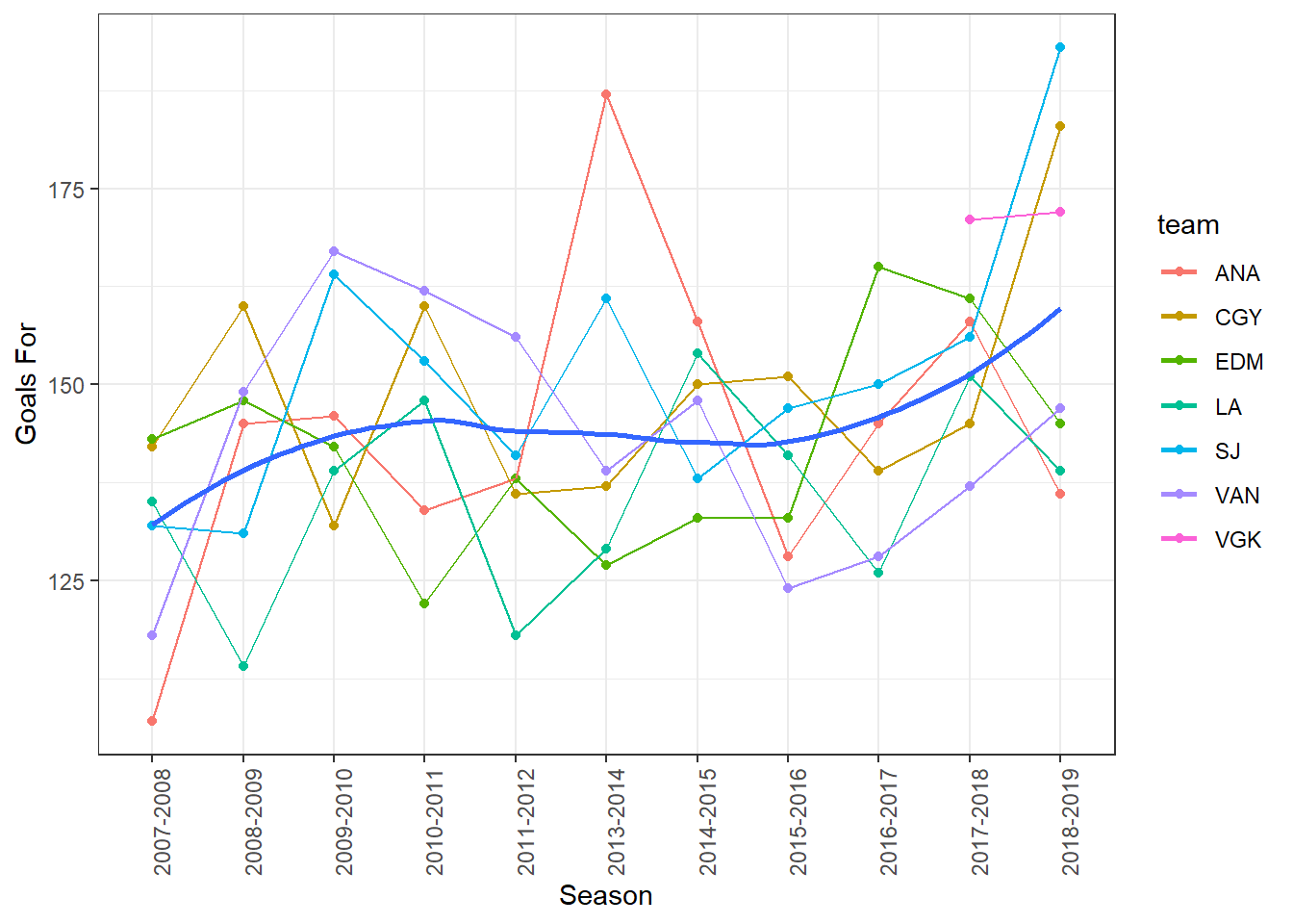
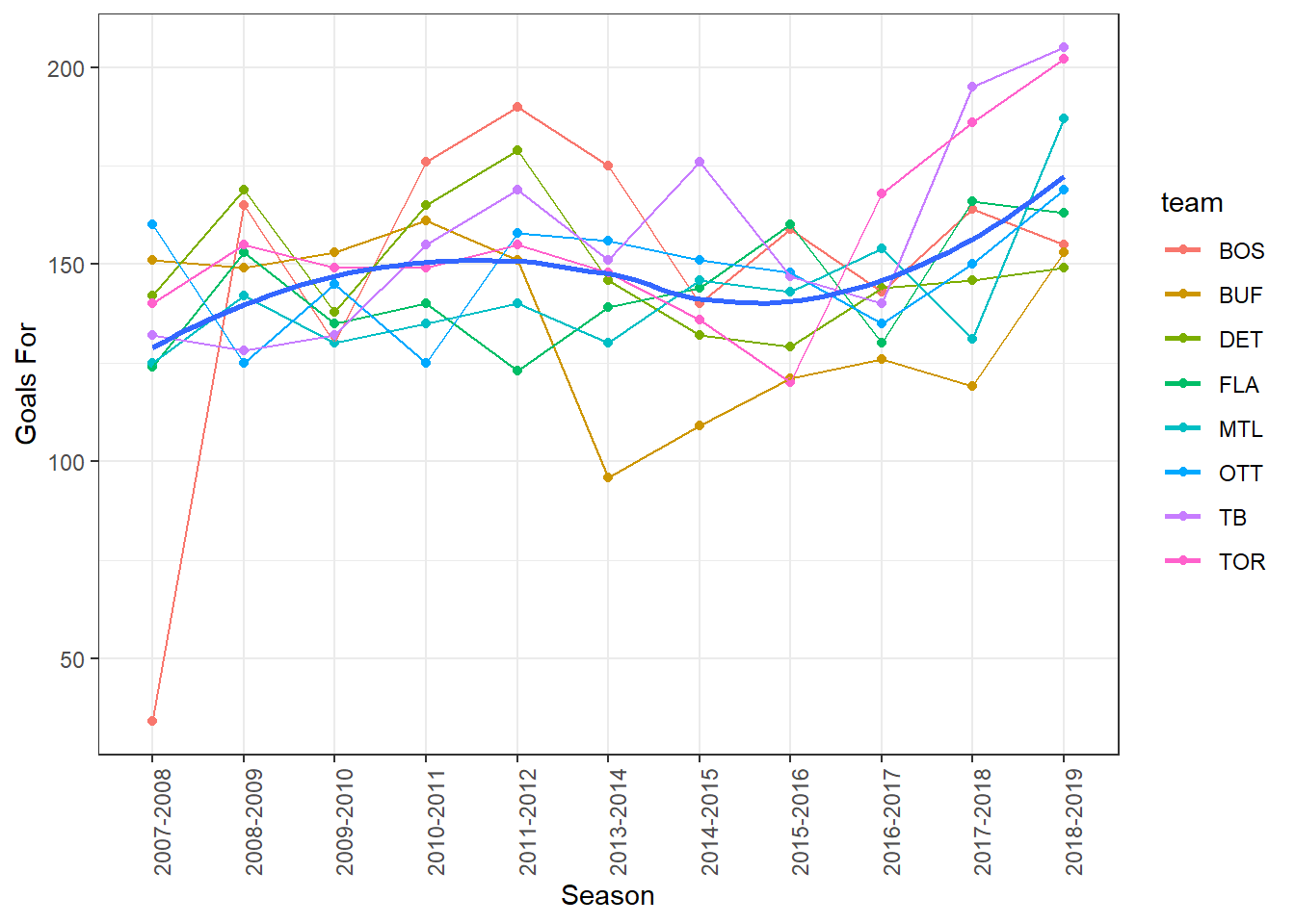
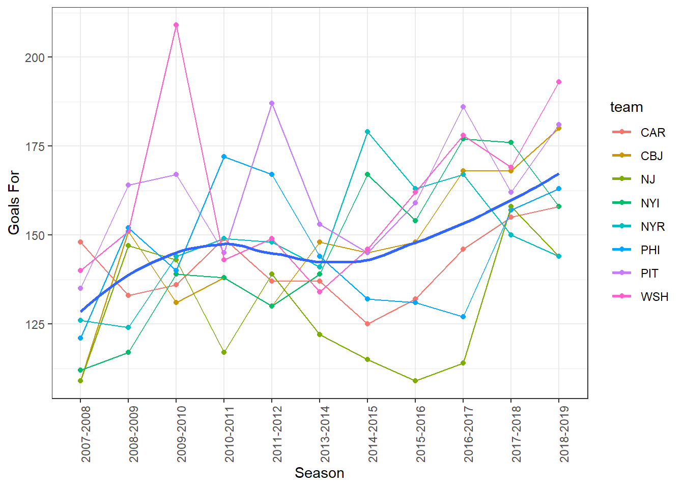
Since we are exploring 5v5, let’s see how important it is by looking at each teams goals for.
Code
Central_div %>%
  filter(season != "2012-2013") %>%
  ggplot(aes(x = season, y = gf, color = team)) +
    geom_point() +
    geom_line(aes(group = team)) +
    geom_smooth(aes(group = 1), se = FALSE) +
    theme_bw() +
    theme(axis.text.x = element_text(angle = 90)) +
    labs(x = "Season",
         y = "Goals For")

Pacific_div %>%
  filter(season != "2012-2013") %>%
  ggplot(aes(x = season, y = gf, color = team)) +
    geom_point() +
    geom_line(aes(group = team)) +
    geom_smooth(aes(group = 1), se = FALSE) +
    theme_bw() +
    theme(axis.text.x = element_text(angle = 90)) +
    labs(x = "Season",
         y = "Goals For")

Atlantic_div %>%
  filter(season != "2012-2013") %>%
  ggplot(aes(x = season, y = gf, color = team)) +
    geom_point() +
    geom_line(aes(group = team)) +
    geom_smooth(aes(group = 1), se = FALSE) +
    theme_bw() +
    theme(axis.text.x = element_text(angle = 90)) +
    labs(x = "Season",
         y = "Goals For")

Metro_div %>%
  filter(season != "2012-2013") %>%
  ggplot(aes(x = season, y = gf, color = team)) +
    geom_point() +
    geom_line(aes(group = team)) +
    geom_smooth(aes(group = 1), se = FALSE) +
    theme_bw() +
    theme(axis.text.x = element_text(angle = 90)) +
    labs(x = "Season",
         y = "Goals For")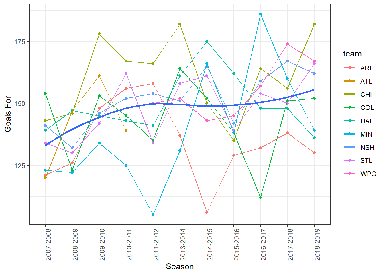
Now let’s look at shot attempts over the years.
Code
Central_div %>%
  filter(season != "2012-2013") %>%
  ggplot(aes(x = season, y = cf/gp, color = team)) +
    geom_point() +
    geom_line(aes(group = team)) +
    geom_smooth(aes(group = 1), se = FALSE) +
    theme_bw() +
    theme(axis.text.x = element_text(angle = 90)) +
    labs(x = "Season",
         y = "Shot Attempts per Game")

Pacific_div %>%
  filter(season != "2012-2013") %>%
  ggplot(aes(x = season, y = cf/gp, color = team)) +
    geom_point() +
    geom_line(aes(group = team)) +
    geom_smooth(aes(group = 1), se = FALSE) +
    theme_bw() +
    theme(axis.text.x = element_text(angle = 90)) +
    labs(x = "Season",
         y = "Shot Attempts per Game")

Atlantic_div %>%
  filter(season != "2012-2013") %>%
  ggplot(aes(x = season, y = cf/gp, color = team)) +
    geom_point() +
    geom_line(aes(group = team)) +
    geom_smooth(aes(group = 1), se = FALSE) +
    theme_bw() +
    theme(axis.text.x = element_text(angle = 90)) +
    labs(x = "Season",
         y = "Shot Attempts per Game")

Metro_div %>%
  filter(season != "2012-2013") %>%
  ggplot(aes(x = season, y = cf/gp, color = team)) +
    geom_point() +
    geom_line(aes(group = team)) +
    geom_smooth(aes(group = 1), se = FALSE) +
    theme_bw() +
    theme(axis.text.x = element_text(angle = 90)) +
    labs(x = "Season",
         y = "Shot Attempts per Game")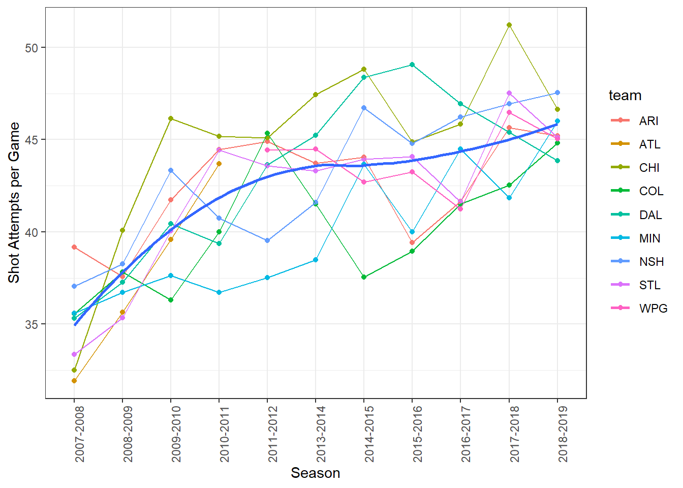
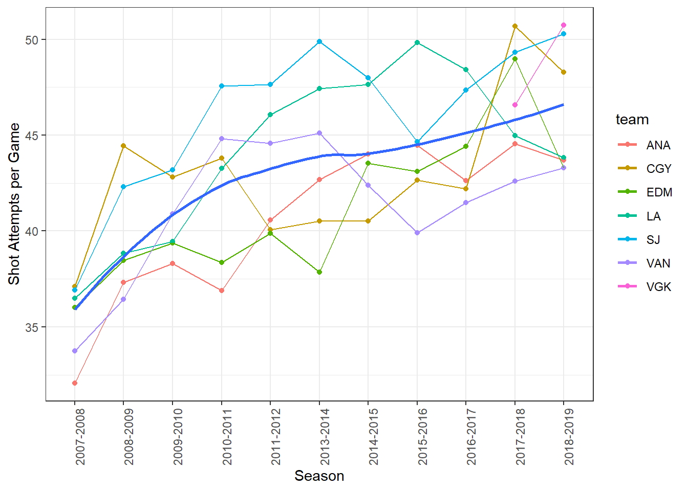
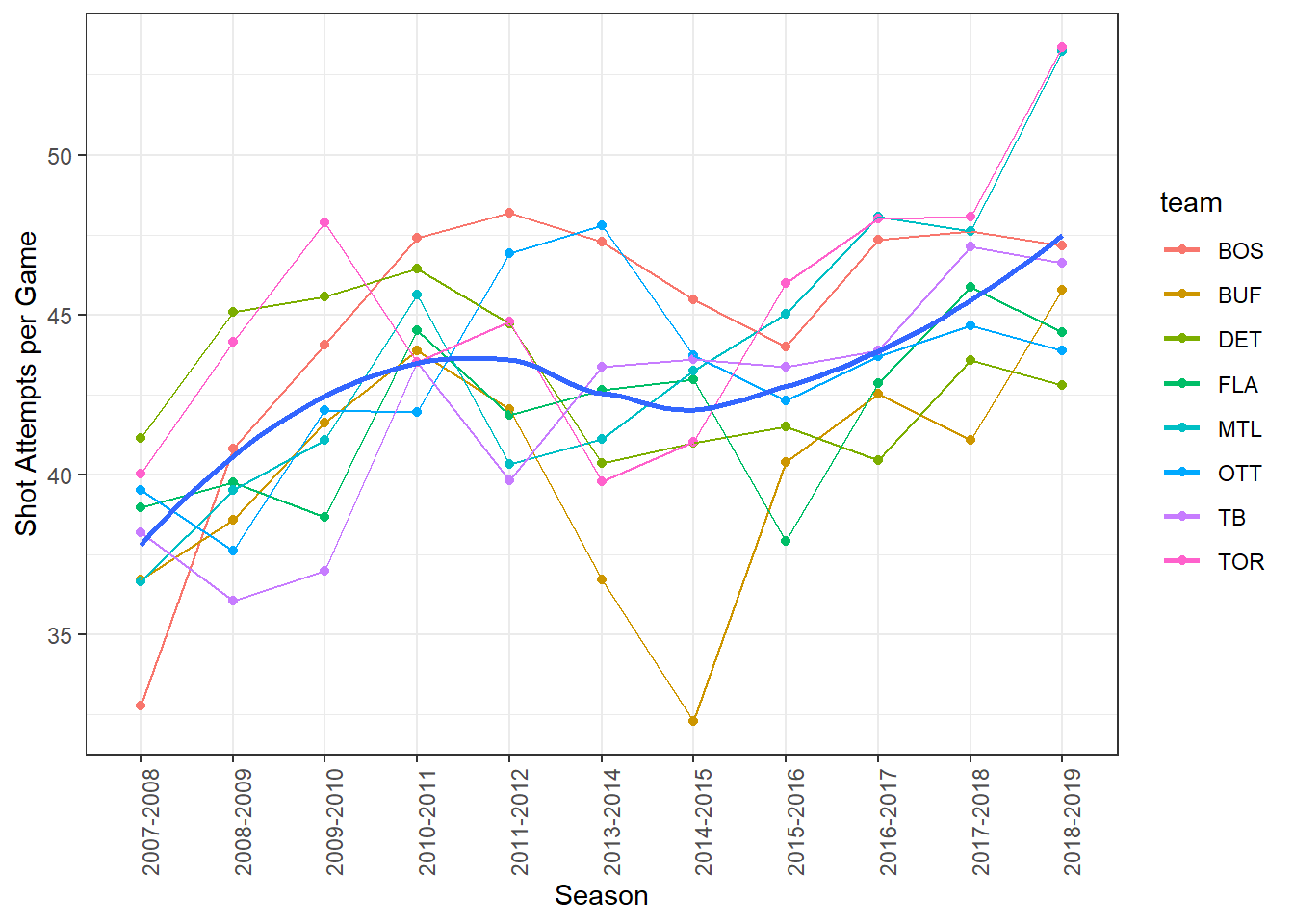
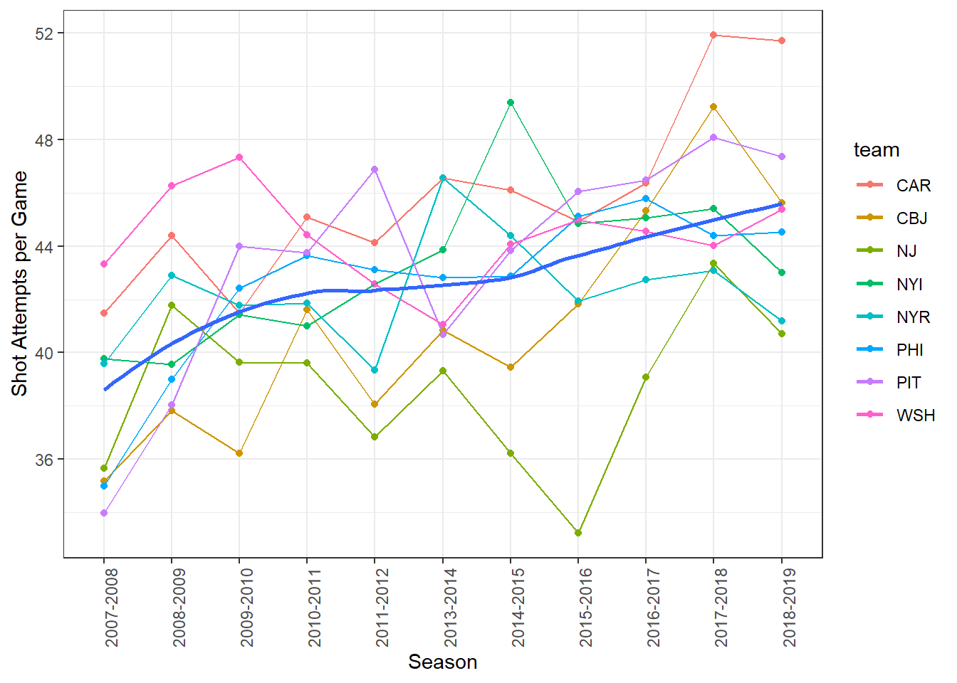
So it looks like there was some fluctuation, but on average teams are scoring slightly more on 5v5 now than they used to and they are attempting more shots per game.
Exploring some data on skaters
glimpse(skaters)Rows: 9,402
Columns: 48
$ player <chr> "SEBASTIAN AHO", "AARON DOWNEY", "AARON EKBLAD", "AARON EK…
$ season <chr> "2017-2018", "2007-2008", "2014-2015", "2015-2016", "2016-…
$ team <chr> "NYI", "DET", "FLA", "FLA", "FLA", "FLA", "FLA", "DAL", "W…
$ team2 <chr> NA, NA, NA, NA, NA, NA, NA, NA, NA, NA, NA, NA, "EDM", NA,…
$ team3 <chr> NA, NA, NA, NA, NA, NA, NA, NA, NA, NA, NA, NA, NA, NA, NA…
$ position <chr> "D", "R", "D", "D", "D", "D", "D", "C", "C", "C", "D", "D"…
$ position2 <chr> "D", NA, NA, NA, NA, NA, NA, NA, NA, NA, NA, NA, NA, NA, N…
$ position3 <chr> "R", NA, NA, NA, NA, NA, NA, NA, NA, NA, NA, NA, NA, NA, N…
$ gp <dbl> 22, 56, 81, 78, 68, 82, 82, 19, 7, 10, 30, 38, 41, 56, 10,…
$ toi <dbl> 324.64, 253.35, 1400.56, 1319.22, 1132.67, 1440.06, 1498.7…
$ g <dbl> 0, 0, 6, 9, 4, 9, 7, 0, 0, 3, 0, 2, 2, 2, 0, 0, 1, 0, 1, 0…
$ a <dbl> 3, 2, 16, 13, 7, 11, 12, 2, 0, 0, 1, 4, 4, 12, 0, 0, 6, 0,…
$ p <dbl> 3, 2, 22, 22, 11, 20, 19, 2, 0, 3, 1, 6, 6, 14, 0, 0, 7, 0…
$ p1 <dbl> 1, 2, 14, 15, 7, 11, 13, 0, 0, 3, 0, 3, 5, 7, 0, 0, 2, 0, …
$ p_60 <dbl> 0.55, 0.47, 0.94, 1.00, 0.58, 0.83, 0.76, 0.84, 0.00, 2.46…
$ p1_60 <dbl> 0.18, 0.47, 0.60, 0.68, 0.37, 0.46, 0.52, 0.00, 0.00, 2.46…
$ gs <dbl> 1.99, 0.92, 38.10, 28.15, 21.36, 19.78, 23.60, 1.64, 1.17,…
$ gs_60 <dbl> 0.37, 0.22, 1.63, 1.28, 1.13, 0.82, 0.94, 0.69, 1.07, 2.83…
$ cf <dbl> 289, 193, 1299, 1059, 1084, 1392, 1402, 127, 72, 64, 287, …
$ ca <dbl> 325, 183, 1112, 1034, 1003, 1520, 1432, 121, 58, 63, 304, …
$ c_plumin <dbl> -36, 10, 187, 25, 81, -128, -30, 6, 14, 1, -17, 28, -83, -…
$ cf_pct <dbl> 47.07, 51.33, 53.88, 50.60, 51.94, 47.80, 49.47, 51.21, 55…
$ rel_cf_pct <dbl> 2.26, -7.30, 3.83, 2.92, 1.97, -2.16, 0.09, 3.14, 8.63, 0.…
$ gf <dbl> 15, 6, 59, 56, 30, 69, 80, 3, 0, 5, 15, 23, 18, 29, 4, 1, …
$ ga <dbl> 19, 6, 43, 43, 47, 67, 82, 6, 1, 4, 11, 10, 25, 37, 4, 0, …
$ g_plumin <dbl> -4, 0, 16, 13, -17, 2, -2, -3, -1, 1, 4, 13, -7, -8, 0, 1,…
$ gf_pct <dbl> 44.12, 50.00, 57.84, 56.57, 38.96, 50.74, 49.38, 33.33, 0.…
$ rel_gf_pct <dbl> -0.48, -12.50, 11.78, -3.07, -7.58, 1.50, 5.93, -11.98, -4…
$ xgf <dbl> 10.49, 7.16, 50.88, 42.44, 38.23, 57.36, 63.91, 5.83, 2.89…
$ xga <dbl> 15.73, 7.76, 42.32, 44.38, 42.23, 65.83, 69.28, 4.84, 2.15…
$ xg_plumin <dbl> -5.24, -0.60, 8.56, -1.94, -4.00, -8.47, -5.37, 0.99, 0.74…
$ xgf_pct <dbl> 40.01, 47.99, 54.59, 48.88, 47.51, 46.56, 47.98, 54.64, 57…
$ rel_xgf_pct <dbl> -3.96, -10.26, 4.30, -0.22, -0.17, -3.54, -0.04, 7.76, 13.…
$ ipent <dbl> 2, 31, 10, 15, 21, 20, 12, 1, 0, 1, 13, 11, 11, 5, 4, 0, 8…
$ ipend <dbl> 4, 15, 10, 6, 13, 9, 9, 0, 0, 1, 4, 5, 5, 7, 1, 1, 4, 0, 2…
$ ip_plumin <dbl> 2, -16, 0, -9, -8, -11, -3, -1, 0, 0, -9, -6, -6, 2, -3, 1…
$ icf <dbl> 50, 22, 229, 208, 248, 271, 227, 25, 12, 17, 33, 53, 70, 9…
$ icf_60 <dbl> 9.24, 5.21, 9.81, 9.46, 13.14, 11.29, 9.09, 10.55, 11.02, …
$ ixgf <dbl> 0.77, 0.94, 3.98, 5.41, 5.59, 6.83, 5.35, 0.84, 0.54, 1.17…
$ ixgf_60 <dbl> 0.14, 0.22, 0.17, 0.25, 0.30, 0.28, 0.21, 0.35, 0.50, 0.96…
$ ish_pct <dbl> 0.00, 0.00, 5.26, 7.50, 2.74, 6.98, 5.56, 0.00, 0.00, 27.2…
$ pdo <dbl> 99.82, 99.80, 100.86, 101.59, 96.77, 100.94, 99.22, 97.67,…
$ zsr <dbl> 43.37, 81.97, 60.73, 55.80, 58.93, 41.48, 45.76, 48.05, 58…
$ toi_pct <dbl> 30.30, 10.37, 36.09, 35.98, 35.20, 36.61, 37.72, 16.25, 18…
$ toi_pct_qot <dbl> 27.25, 26.06, 28.14, 28.15, 27.69, 29.52, 29.32, 26.44, 29…
$ cf_pct_qot <dbl> 47.37, 57.52, 49.53, 48.73, 50.29, 51.68, 49.32, 44.92, 50…
$ toi_pct_qoc <dbl> 28.78, 27.06, 28.56, 28.77, 28.91, 29.52, 29.89, 28.06, 28…
$ cf_pct_qoc <dbl> 50.10, 48.87, 49.31, 49.94, 50.02, 50.12, 50.19, 50.72, 48…There are 48 variables in the skaters data set:
Note: Corsi stat in hockey is Shot attempts
player: Player nameseason: Seasonteam: First team player played for in a given seasonteam2: Second team player played for in a given seasonteam3: Third team player played for in a given seasonposition: Player’s first positionposition2: Player’s second positionposition3: Player’s third positiongp: Games Playedtoi: Time on the iceg: Goals scoreda: Assistsp: Pointsp1: Primary points (goals + primary assists)p_60: Points per 60 minutes on the icep1_60: Primary points per 60 minutes on the icegs: Game scoregs_60: Game score per 60 minutes on the icecf: Corsi for (shot attempts by player’s team while player is on the ice)ca: Corsi against (shot attempts by opposing team will player is on the ice)c_plumin: Corsi plus/minus (cf-ca)cf_pct: Corsi percentagerel_cf_pct: Relative corsi percentagegf: Goals scored for a player’s teamga: Goals scored against player’s teamg_plumin: Shooting Goals for - goals againstgf_pct: Save Percentage of all goals scored by player’s teamrel_gf_pct: Relative goals for percentagexgf: Expected goals forxga: Expected goals againstxg_plumin: Expected goals for - expected goals againstxgf_pct: Expected goals for as a percentage of a team’s total expected goals forrel_xgf_pct: Relative expected goals for as a percentage of a team’s total expected goals foripent: Individual penalties takenipend: Individual penalties drawnip_plumin: Individual penalties taken - individual penalties drawnicf: Individual corsi foricf_60: Individual corsi for per 60 minutes on the iceixgf: Individual expected goals forixgf_60: Individual expected goals for per 60 minutes on the iceish_pct: Individual shooting percentagepdo: Just Win Babyzsr: Zone start ratiotoi_pct: Percentage of team’s total time on ice played by playertoi_pct_qot: Percentage of team’s total time on ice played by player, weighted by quality of teammatescf_pct_qot: Corsi for percentage weighted by quality of player’s teammatestoi_pct_qoc: Percentage of team’s total time on ice played by player, weighted by quality of opponentscf_pct_qoc: Corsi for percentage weighted by quality of player’s opponents
It would be nice to see if the individual player stats reflect this slight increase in production.
Code
skaters %>%
  filter(season != "2012-2013") %>%
  filter(p >= 50) %>%
  ggplot(aes(x = season)) +
    geom_bar(color = "black", fill = "lightblue") +
    theme_bw() +
    theme(axis.text.x = element_text(angle = 90)) +
    labs(x = "Season",
         y = "Count")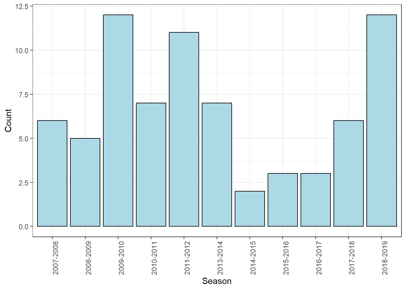
Code
skaters %>%
  filter(season != "2012-2013") %>%
  filter(ish_pct >= 20) %>%
  ggplot(aes(x = season)) +
  geom_bar(color = "black", fill = "lightblue") +
  theme_bw() +
  theme(axis.text.x = element_text(angle = 90)) +
    labs(x = "Season",
         y = "Count")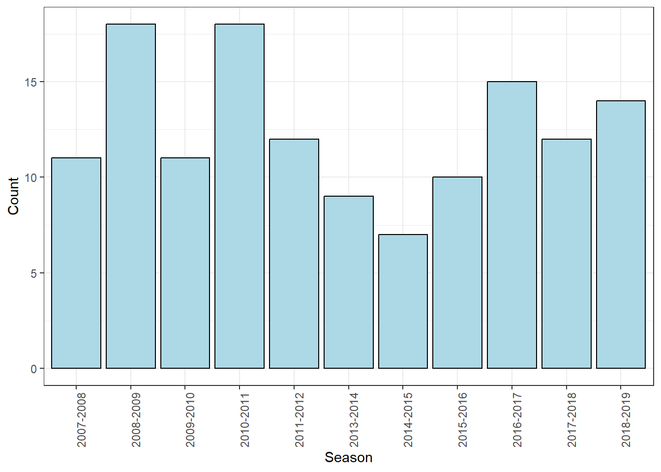
Code
skaters %>%
  filter(season != "2012-2013") %>%
  filter(ish_pct >= 10) %>%
  ggplot(aes(x = season)) +
  geom_bar(color = "black", fill = "lightblue") +
  theme_bw() +
  theme(axis.text.x = element_text(angle = 90)) +
    labs(x = "Season",
         y = "Count")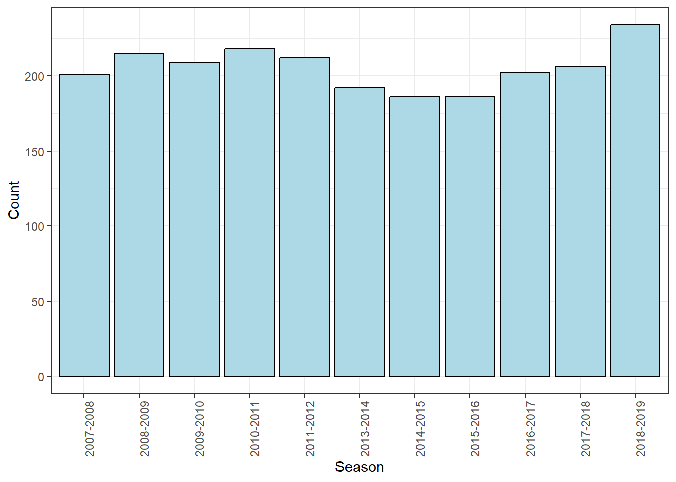
Interesting, the amount of players with at least 50 points seems to be trending up in the last couple of years but is not more than some of the years in the past. Also shooting percentage has stayed relatively consistent, but at 20% there were some spikes.
Exploring some data on goalies
glimpse(goalies)Rows: 856
Columns: 16
$ player <chr> "AARON DELL", "AARON DELL", "AARON DELL", "ADIN HILL", "ADIN …
$ season <chr> "2016-2017", "2017-2018", "2018-2019", "2017-2018", "2018-201…
$ team <chr> "SJ", "SJ", "SJ", "ARI", "ARI", "NYR", "NYR", "ARI", "OTT", "…
$ team2 <chr> NA, NA, NA, NA, NA, NA, NA, "BOS", NA, "NYR", NA, NA, NA, NA,…
$ team3 <chr> NA, NA, NA, NA, NA, NA, NA, NA, NA, NA, NA, NA, NA, NA, NA, N…
$ gp <dbl> 20, 29, 25, 4, 13, 10, 33, 32, 43, 24, 16, 14, 11, 24, 22, 13…
$ toi <dbl> 951.31, 1235.49, 1057.78, 205.05, 545.18, 430.98, 1486.20, 12…
$ sa <dbl> 449, 606, 473, 113, 255, 274, 822, 534, 823, 472, 278, 215, 1…
$ ga <dbl> 23, 49, 45, 12, 25, 19, 69, 41, 64, 46, 24, 20, 18, 31, 41, 2…
$ sv_pct <dbl> 94.88, 91.91, 90.49, 89.38, 90.20, 93.07, 91.61, 92.32, 92.22…
$ xsv_pct <dbl> 92.44, 91.74, 91.24, 90.27, 91.73, 91.86, 91.76, 92.30, 92.14…
$ dsv_pct <dbl> 2.43, 0.17, -0.75, -0.88, -1.54, 1.21, -0.15, 0.02, 0.08, -2.…
$ ldsv_pct <dbl> 98.64, 97.60, 98.03, 91.67, 95.76, 99.24, 98.06, 97.22, 98.67…
$ mdsv_pct <dbl> 96.03, 92.97, 89.02, 93.75, 94.94, 89.77, 91.17, 92.24, 90.23…
$ hdsv_pct <dbl> 82.05, 77.52, 78.30, 81.82, 72.41, 83.64, 79.33, 80.23, 83.06…
$ gsaa <dbl> 10.93, 1.05, -3.57, -1.00, -3.92, 3.31, -1.23, 0.12, 0.65, -1…There are 16 variables in the teams data set:
player: Player nameseason: Seasonteam: First team player played for in a given seasonteam2: Second team player played for in a given seasonteam3: Third team player played for in a given seasongp: Games Playedtoi: Time on the icesa: Shots againstga: Goals againstsv_pct: Save percentagexsv_pct: Expected save percentagedsv_pct: Dangerous save percentageldsv_pct: Low danger save percentagemdsv_pc: Medium danger save percentagehdsv_pct: High danger save percentagegsaa: Goals saved above average
How have the goalies been affected over the years?
Code
goalies %>%
  filter(season != "2012-2013") %>%
  filter(sv_pct >= 91.00) %>%
  filter(gp >= 45) %>%
  ggplot(aes(x = season)) +
  geom_bar(color = "black", fill = "pink") +
  theme_bw() +
  theme(axis.text.x = element_text(angle = 90)) +
    labs(x = "Season",
         y = "Count")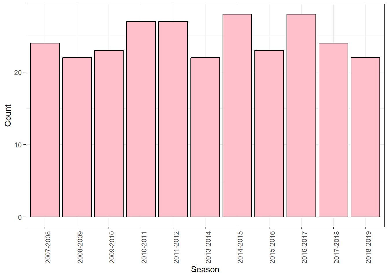
Code
goalies <- goalies %>%
  mutate(avg_sa_gp = sa/gp)

filtered_goalies <- goalies %>%
  filter(season != "2012-2013") %>%
  filter(gp > 5) %>%
  filter(avg_sa_gp >= 20)

ggplot(filtered_goalies, aes(x = season)) +
  geom_bar(color = "black", fill = "pink") +
  theme_bw() +
  theme(axis.text.x = element_text(angle = 90)) +
    labs(x = "Season",
         y = "Count")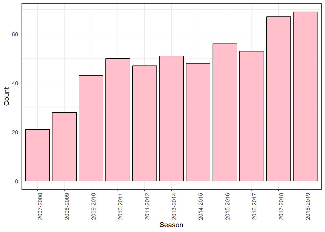
Looking at penalties
Code
Central_div %>%
filter(season != "2012-2013") %>%
ggplot(aes(x = season, y = pent, color = team)) +
geom_point() +
geom_line(aes(group = team)) +
geom_smooth(aes(group = 1), se = FALSE) +
theme_bw() +
theme(axis.text.x = element_text(angle = 90)) +
labs(x = "Season",
y = "Penalties Taken")
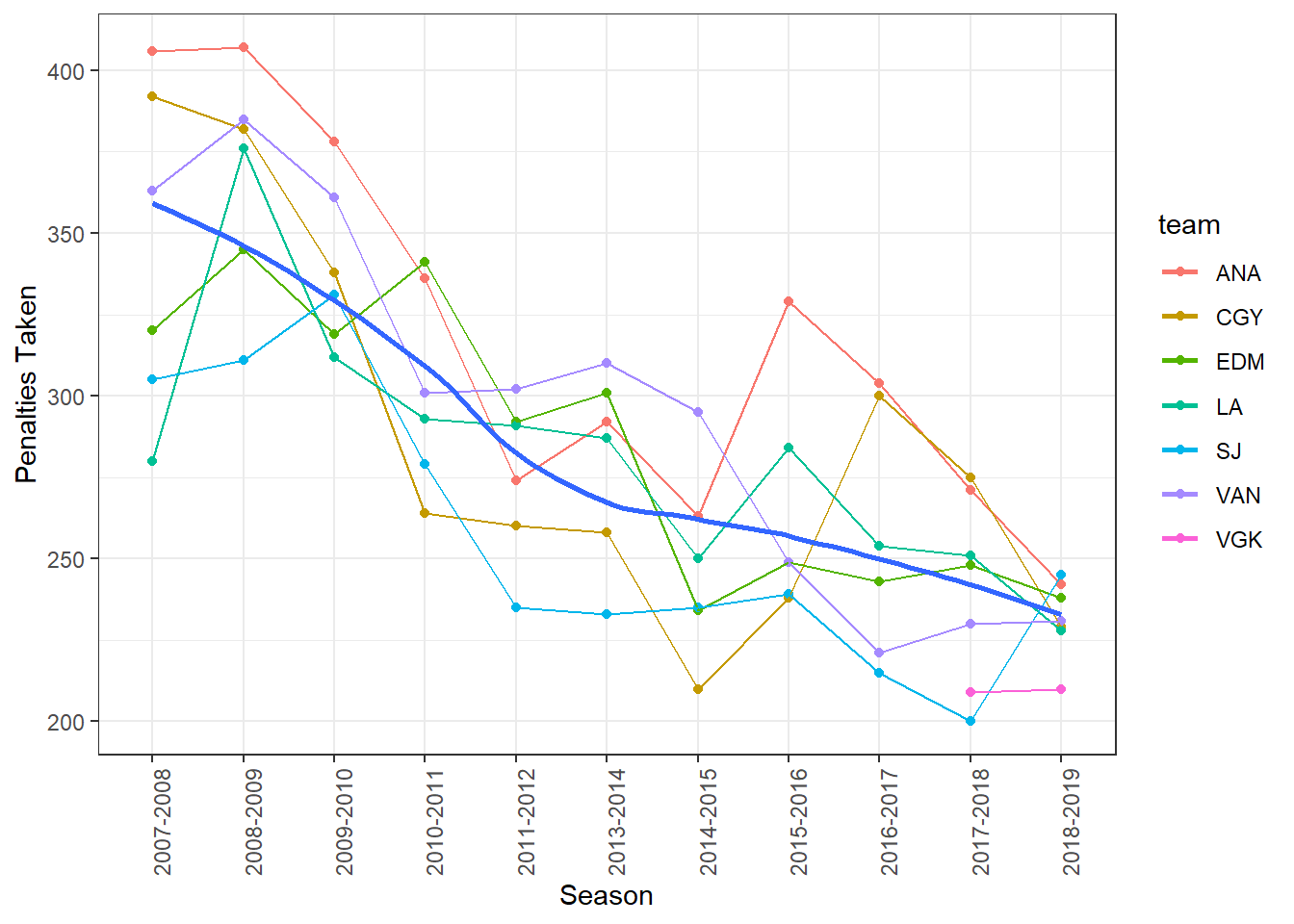
Pacific_div %>%
filter(season != "2012-2013") %>%
ggplot(aes(x = season, y = pent, color = team)) +
geom_point() +
geom_line(aes(group = team)) +
geom_smooth(aes(group = 1), se = FALSE) +
theme_bw() +
theme(axis.text.x = element_text(angle = 90)) +
labs(x = "Season",
y = "Penalties Taken")
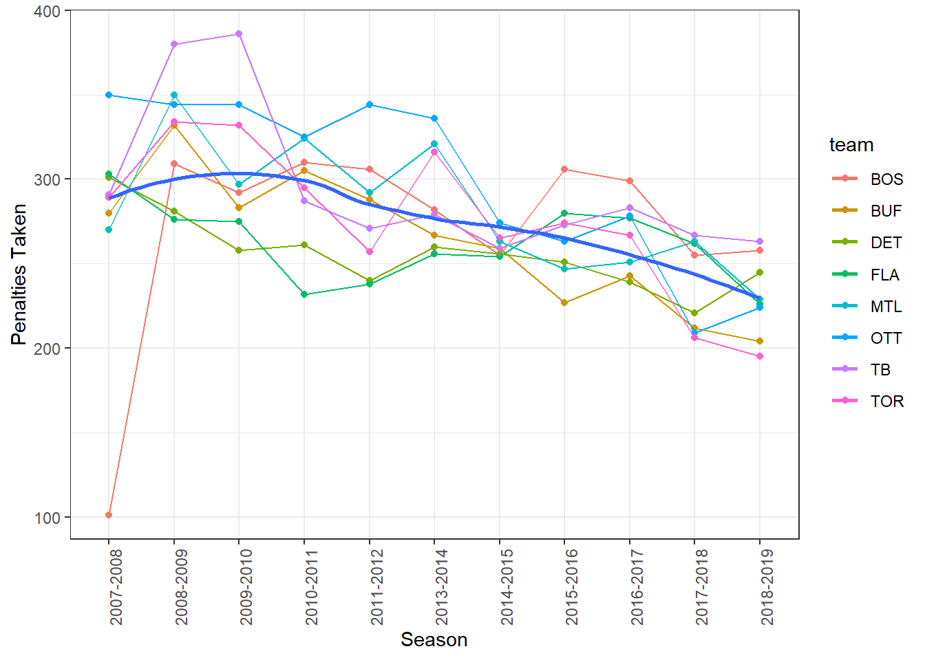
Atlantic_div %>%
filter(season != "2012-2013") %>%
ggplot(aes(x = season, y = pent, color = team)) +
geom_point() +
geom_line(aes(group = team)) +
geom_smooth(aes(group = 1), se = FALSE) +
theme_bw() +
theme(axis.text.x = element_text(angle = 90)) +
labs(x = "Season",
y = "Penalties Taken")
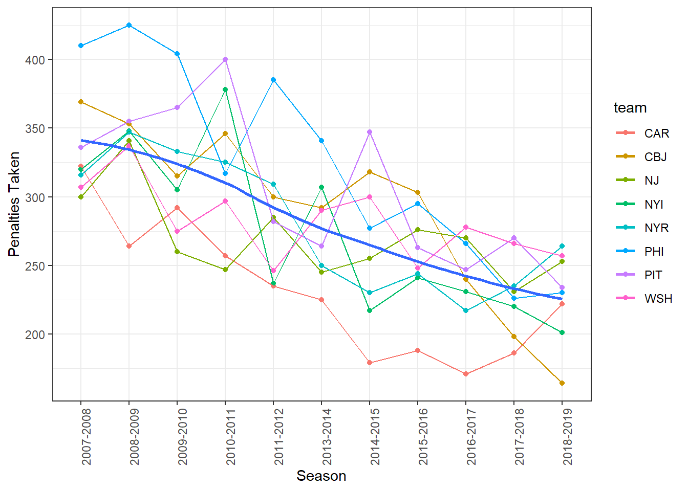
Metro_div %>%
filter(season != "2012-2013") %>%
ggplot(aes(x = season, y = pent, color = team)) +
geom_point() +
geom_line(aes(group = team)) +
geom_smooth(aes(group = 1), se = FALSE) +
theme_bw() +
theme(axis.text.x = element_text(angle = 90)) +
labs(x = "Season",
y = "Penalties Taken")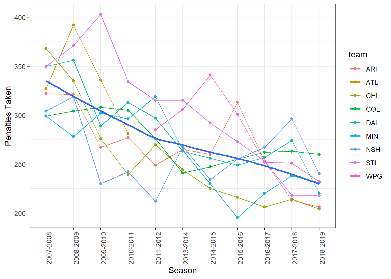
Code
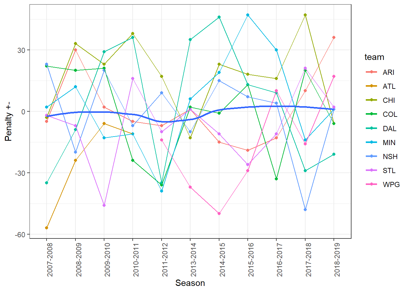
Central_div %>%
filter(season != "2012-2013") %>%
ggplot(aes(x = season, y = p_plumin, color = team)) +
geom_point() +
geom_line(aes(group = team)) +
geom_smooth(aes(group = 1), se = FALSE) +
theme_bw() +
theme(axis.text.x = element_text(angle = 90)) +
labs(x = "Season",
y = "Penalty +-")
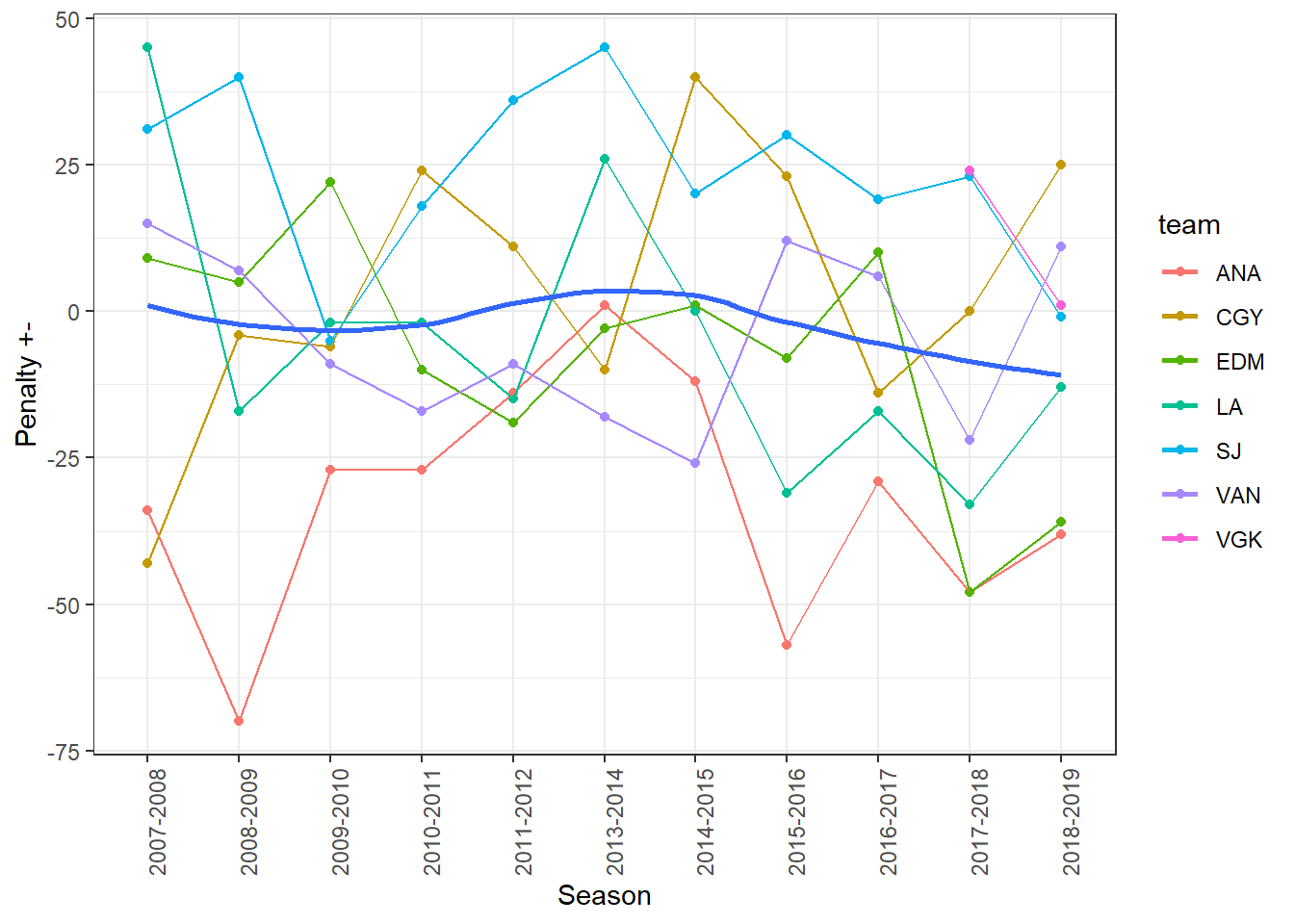
Pacific_div %>%
filter(season != "2012-2013") %>%
ggplot(aes(x = season, y = p_plumin, color = team)) +
geom_point() +
geom_line(aes(group = team)) +
geom_smooth(aes(group = 1), se = FALSE) +
theme_bw() +
theme(axis.text.x = element_text(angle = 90)) +
labs(x = "Season",
y = "Penalty +-")
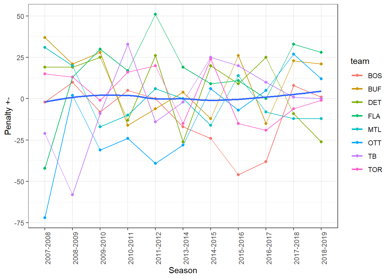
Atlantic_div %>%
filter(season != "2012-2013") %>%
ggplot(aes(x = season, y = p_plumin, color = team)) +
geom_point() +
geom_line(aes(group = team)) +
geom_smooth(aes(group = 1), se = FALSE) +
theme_bw() +
theme(axis.text.x = element_text(angle = 90)) +
labs(x = "Season",
y = "Penalty +-")
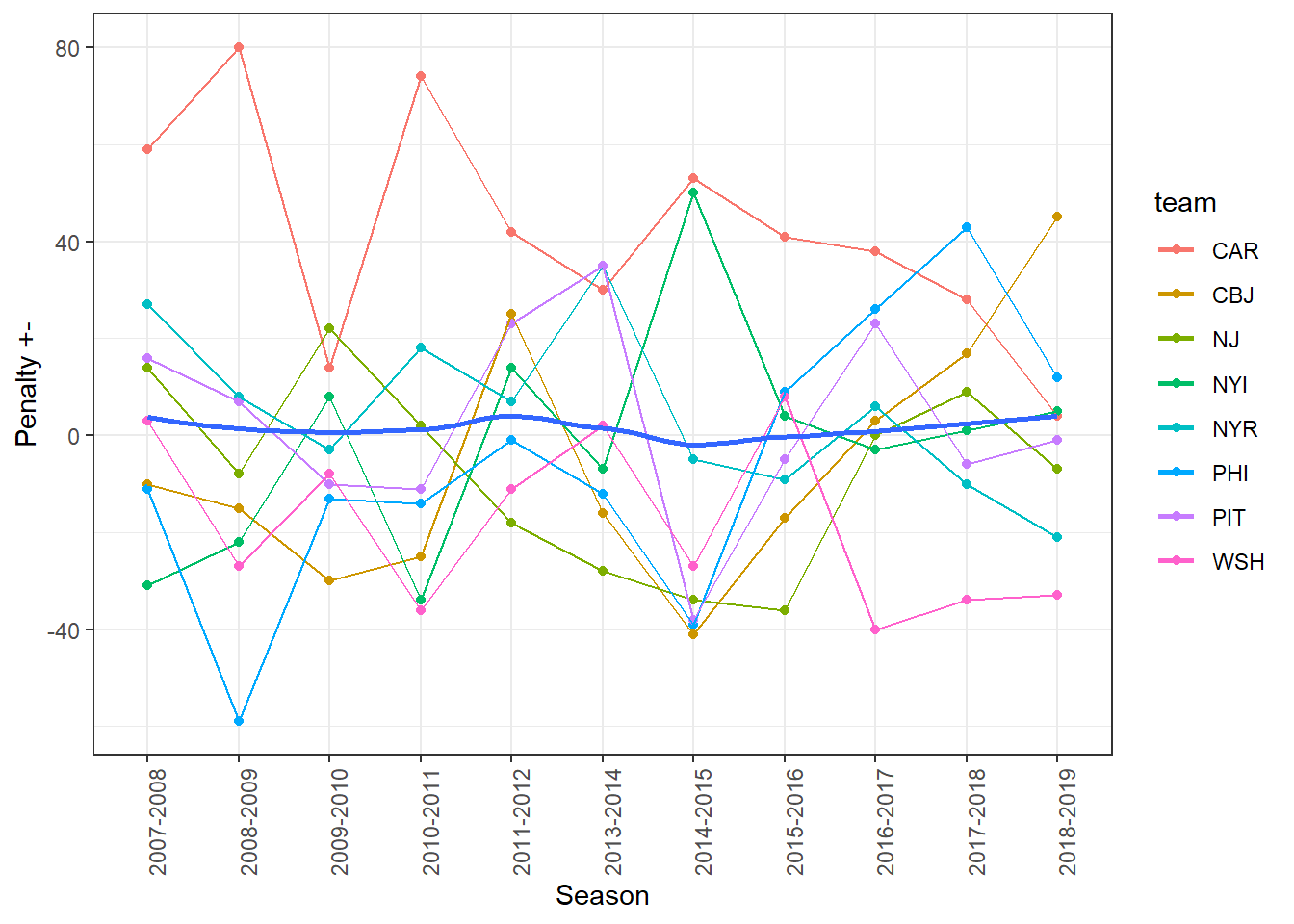
Metro_div %>%
filter(season != "2012-2013") %>%
ggplot(aes(x = season, y = p_plumin, color = team)) +
geom_point() +
geom_line(aes(group = team)) +
geom_smooth(aes(group = 1), se = FALSE) +
theme_bw() +
theme(axis.text.x = element_text(angle = 90)) +
labs(x = "Season",
y = "Penalty +-")